Running INCInERATOr on a Kepler Target¶

In this tutorial, we will learn how to use incinerator!

Step 1: Imports¶

First, make sure you are running the notebook in the correct environment (if you created one). Your Python kernel should be set to that environment.

Next, import incinerator and a few other useful packages.

import pandas as pd
from astropy.io import fits

import incinerator.localize as loc

%matplotlib inline

Step 2: Initialize Localize Object¶

NOTE: `incinerator` can now handle observations from multiple epochs using the `Multi_Localize` class. An udated tutorial notebook showing this feature is coming soon!¶

Get Your File¶

For this tutorial, we will use the Quarter 1 target pixel file (TPF) for Kepler-8 (KIC 6922244).

⚠️ Important: incinerator requires a local file when using Kepler or TESS TPFs, because it relies on information in the .fits header.

You have two options:

1. Download manually

You can download the TPF from MAST Kepler Search.

2. Download using astroquery

You will need to add the following to your imports:

from astroquery.mast import Observations


```python
#you can find the file in the tutorials/` folder inside the `docs/` directory on GitHub.
file_path = "kplr006922244-2009166043257_lpd-targ.fits"
#opening the file
hdu = fits.open(file_path)

#extracting time, flux cube (in this case a tpf), and flux cube error
time = hdu[1].data['TIME']
flux = hdu[1].data['FLUX']
flux_err = hdu[1].data['FLUX_ERR']

Load Your TCEs¶

You will also need the information for the Threshold Crossing Events (TCEs).

You have two options:

1. Read from a CSV file

2. Create a pandas DataFrame manually

Note: Kepler-8 only has one TCE, but if your target has multiple TCEs, you can simply add each of them as a row in the same DataFrame.

Important: Make sure the dataframe includes the columns:

period → in units of days
t0 → in BJD
tdur → best rounded to two significant figures and in units of days

#creating tce dataframe
tces = pd.DataFrame({'star_id':6922244.01,
                     'period':3.5224,
                     't0':121.1194228+2454833,
                     'tdur':.12},index=[0])

Initialize the Localize Object¶

Now it’s time to create a Localize object!

You will need to provide the following inputs:

time → 1D array of time values in BJD
flux → 3D flux cube
flux_err → 3D array of per-pixel uncertainties
tces → TCE DataFrame containing period, t0, and tdur
id → target's identifier (ie KIC or TIC)
ra_targ, dec_targ → target coordinates in degrees
wcs → WCS solution for pixel-to-sky transformations
epoch → epoch of the input coordinates

Optional: If you are analyzing a background star in the TPF, you can also include bonus RA and DEC.

If these inputs are already available, you can initialize the object directly:

loc_obj = loc.Localize(time=time, flux=flux, flux_err=flux_err, tces=tces, 
                    id='6922244', ra_targ=ra_targ, dec_targ=dec_targ, 
                    wcs=wcs, epoch=epoch, mission='kepler')

When starting from a Kepler or TESS TPF, the static method can load these inputs automatically:

loc_obj = loc.Localize.from_tpf_info(file_path,tces,'6922244',mission='kepler')

#initialize you Localize class object
loc_obj = loc.Localize.from_tpf_info(file_path,tces,'6922244',mission='kepler')

/Users/jmoquin/mypy/incinerator/.venv/lib/python3.11/site-packages/erfa/core.py:133: ErfaWarning: ERFA function "pmsafe" yielded 4 of "distance overridden (Note 6)"
  warn(f'ERFA function "{func_name}" yielded {wmsg}', ErfaWarning)
/Users/jmoquin/mypy/incinerator/.venv/lib/python3.11/site-packages/erfa/core.py:133: ErfaWarning: ERFA function "pmsafe" yielded 1 of "distance overridden (Note 6)"
  warn(f'ERFA function "{func_name}" yielded {wmsg}', ErfaWarning)

This is the recommended approach when working directly from a TPF.

See the API documentation for the complete list of parameters.

Step 3: Build the Design Matrix¶

Now we get to the easier part: running the necessary functions.

We need to build the design matrix, which incorporates all of the TCEs in your DataFrame.

#build the design matrix
loc_obj.build_design_matrix()

incinerator now supports a batman transit model in addition to the box model. The transit model can be selected using the transit_method parameter. When using batman, you will need to provide precomputed model parameters (e.g., \(R_p\), limb darkening coefficients, and inclination) for each TCE.

Step 4: Generate Heatmaps and Fit PRF¶

Solve for the transits¶

First, we solve for the weights of each transit component in the design matrix.

If your target has multiple TCEs, they are solved simultaneously.

#solve for the weights of the transit components
loc_obj.solve_transit_weights()

/Users/jmoquin/mypy/incinerator/src/incinerator/localize.py:531: RuntimeWarning: invalid value encountered in sqrt
  self.weights_err[idx] = np.sqrt(np.diag(np.linalg.inv(sigma_w_inv)))

Fit PRF model¶

Next, we fit the PRF model to the resulting heat map to determine the likely location of the signal on the CCD.

If your target has multiple TCEs, you have two options:

1. Fit all TCEs at once

  which_tce = None

2. Fit one TCE at a time

  which_tce = <index of the TCE>

#fit prf to heatmap
full_report, fit = loc_obj.fit_to_heatmap(method='prf',which_tce=0)
full_report

Fit Result

Fit Statistics
fitting method	leastsq
# function evals	48
# data points	35
# variables	3
chi-square	975.053016
reduced chi-square	30.4704067
Akaike info crit.	122.450032
Bayesian info crit.	127.116077

Parameters
name	value	standard error	relative error	initial value	max	vary
centery	2.20424801	0.02157443	(0.98%)	2.1904447560534286	5.00000000	True
centerx	2.83480228	0.01766358	(0.62%)	2.7563988033219746	5.00000000	True
amplitude	384.896472	8.29757202	(2.16%)	98.6776473117501	inf	True

By default, fit_to_heatmap() initializes the fit at the target's catalog position, using ra_bonus/dec_bonus when available and otherwise ra_targ/dec_targ. If a better estimate of the source location is known, an initial pixel location can be provided with initial_loc=(col, row):

Step 5: Visualize Results¶

Plot the results¶

#getting the incinerator report
loc_obj.plot_heatmap(fit,0,savefig=False)

/Users/jmoquin/mypy/incinerator/src/incinerator/localize.py:901: RuntimeWarning: Mean of empty slice
  cax1 = axes[0].imshow(np.nanmean(self.flux, axis=0),origin='lower')

png

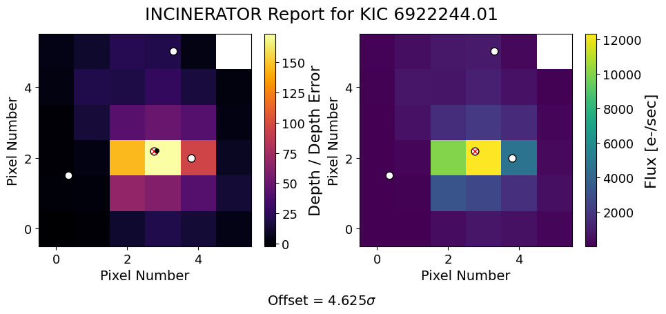
Interpreting results¶

The output figure contains two panels:

Left panel: The Target Pixel File (TPF)
Right panel: The "transit localization" heatmap
The red X marks the star of interest.
The black dot shows the fitted location of the transit signal.
Error bars represent the uncertainty in the fitted position.

The localization results include several metrics describing the separation between the fitted position and the position of the star of interest: - Euclidean distance: The distance between the fitted and star-of-interest positions in pixels. - Euclidean distance error: The uncertainty in the Euclidean distance. - Offset: The Euclidean distance divided by its uncertainty, expressed in units of \(\sigma\). - Mahalanobis distance: A two-dimensional measure of the separation that accounts for the uncertainties in both coordinates and their covariance.

If the fitted position is close to the pixel containing the star of interest, this suggests the transit signal is likely originating from that pixel. Larger offsets may indicate that the signal is coming from a nearby contaminating source instead.